Demo

Demo

Demo

The Basics

In RLP, an object is defined as a stream of bytes. A nested data structure is an object and it is composed of a sequence of objects too. This is formally defined in the yellow paper with equations 178 to 180.

Here, $\mathbb{T}$ is the set of all possible nested data structures, $\mathbb{L}$ is the set of all sequences of data structures and $\mathbb{B}$ is the set of all sequences of bytes ($\mathbb{O}$ is the set of all possible bytes). As the name suggests, an nested data structure is recursive and so is its definition.

All in all, these formulas elegantly define what an RLP object is. RLP is meant to serialize the object into a new object that would belong to $\mathbb{B}$. In order to achieve this, a form of protocol needs to be conceived. It would be used to encode and decode the data structure.

The Protocol

Before looking at the protocol, let us think about how one would encode a nested data structure into a byte stream.

Given the definitions of the previous section, a nested data structure is essentially a list of objects of the same nature as the one being describe with this sentence. The recursion stops when the object is no longer a list of objects but rather an explicit list of bytes. Similarly, a nested data structure could be viewed as a tree of objects. A leaf is a list of bytes whereas any non-leaf nodes are list of abstract objects. This distinction must be reflected in the protocol. When encoding, one must recursively encode objects until a leaf (list of bytes) is encountered and explicitely label that branch as being a leaf. This is usually done using a header to the actual data. When decoding, this header would be used to know how to interpret the data.

In Ethereum, equations 181 to 186 make this distinction. If you have taken the time to look at the different cases in those formulas, you have probably wondered why is there an additional distinction between short leaves, long leaves, short objects and long objects. This is because RLP aims to minimize the amount of bytes for the encoding. It can be particularly useful if the objects to serialize are small but numerous.

The author of RLP decided to use a single byte for the header. The catch is that since there are only two cases to the encoding (a leaf or a non leaf), most of the values that a byte can take remain unused. A single bit would have sufficed. That being said, since the byte is the smallest unit representable in a machine, we are stuck with it. The author decides to use the remaining values for very small sequences.

A leaf that is a single byte long is encoded in the header immediately as long as its value is lower than 128. Then, for leaves of length smaller than 56, the size is encoded into the header and it is concatenated with the data. Finally, for anything longer or equal to 56 bytes, up to 8 extra bytes are used to encode the length and the amount of these bytes is encoded in the header.

For non-leaves, objects that are at most 56 bytes long have their length encoded in the header. For longer objects, up to 8 bytes are used to encode their size and the amount of these bytes is encoded in the header. In this case, the data is a concatenation of the RLP encoding of each children node.

These choices may look odd but they are made in the goal of minimizing the amount of bytes of the encoding. A simpler protocol could be devised where each object uses a byte to distinct leaves from non leaves and 8 bytes to represent the size. This protocol would end up using a lot more bytes than RLP. Here is a figure that shows the amount of bytes used by RLP and a more naive protocol:

makes the distinction between a short object and a long object.

Performance

At first glance, the recursive prefixing of the data with a header is severely inneficient. As a matter of fact, if a regular string like object is used and if headers are appended using new copies, every byte in a leaf will be written $O(h) \equiv O(\log{n})$ times, where $h$ is the height of the tree and $n$ is the number of nodes in the tree. All in all, the encoding would take about $O(n\log{n})$ time. This can be made more efficient. The fact that arrays grow from left to right is a simple programming choice. One could use reverse arrays (writting the data and the header in the reverse order and dropping the header after the data and reversing the whole byte array at the end) or right to left growing arrays. The resulting time complexity would end up being $\Theta(n)$.

Conclusion

RLP is not so difficult to understand. The constants were chosen with space minimization in mind.

References

• Wood, Gavin. (2020-09-05). Ethereum: A Secure Decentralised Generalised Transaction Ledger. Petersburg Version.

Assuming we are coding in C or C++, generally, when implementing linked lists, one would rely on the power of macros or templates to abstract types. It is also possible to abstract types with raw pointers to hold the data but that comes with the cost of an extra indirection which may affect performance. Until now, I did not know any other way of creating a convenient, type abstracted linked list (if you hate macros, templates and raw pointers, you could even go as far as defining an opaque structure with a size field but it is way too ugly for my liking).

Essentially, the goal of these methods was to define some kind of structure that would hold a pointer to anoter same structure. That would make this chain a linked list. It would look a little bit like this:

template<typename T>
struct ListNode {
    T data;
    Node *next;
    Node *prev;
};

But there is a fundamental flaw with this approach: it strongly assumes lists should point to the same type that holds them whereas in reality, the only requirement to have a linked list would be to somehow connect objects and have a way of deleting and ading more objects in the chain. In a way, linked lists already use indirection and that assumptions did not take advantage of it.

Intrusive linked lists, on the other hand, aim to define a simple structure that will be embedded inside a user structure (hence the name). It does precisely what a linked list is supposed to do: act like a pointer.

// Simple list structure that is meant to be embedded into a user struct.
struct list {
    struct list *next;
    struct list *prev;
};

// User defined structure
struct UserStruct {
    int data
    size_t len;
    ...
    struct list list;
    ...
};

This representation has several advantages:

1. Firstly, we achieve type abstraction without the use of macros (they’re highly inconvenient) or templates (if you’re stuck with C). The only macro required for this kind of list is the offsetof which is already provided by gcc. This is necessary to get the data associated with a list node. An implementation would look like:

   #define offsetof(name, type) (&((type*)0)->name))
   

2. Secondly, because it does not rely on macros nor templates to redefine every procedure for every type, the code size is generally smaller. This could be useful for very restricted systems. Such procedures involve the initialization of the list and add and remove operations.

   void list_add(struct list *parent, struct list *child)
   {
    if (parent->next)
    {
        parent->next->prev = child;
    }
    child->next = parent->next;
    parent->next = child;
    child->prev = parent;
   }
   

3. Futhermore, This kind of representation could be applied to any pointer based data structure like trees or graphs. The only downside is that if there is ever a requirement to sort or operate on the data, comparators will not be inlined.
4. Finally, it is possible to have a heterogeneous list because the type is, again, not assumed with this representation. The type identifier must be at a constant offset from the list structure in this case. Alternatively, the list structure could be set as the first field of the list node (an offset of 0 bytes).

   struct UserStruct {
    struct list list;
    int type_id;
    ...
   };
   

I was made aware of this when I stumbled upon Linux data structures. Unlike C++, C does not have a standard library for general purpose data structures and algorithms (you could always use gnulib but that comes at a very strong assumptions that you are using autotools. glib is a good choice though.) and so I wondered how did the kernel writers achieve anything down there.

The time taken by quicksort can be modeled by the following recurrence:

Note that an ideal split would be when $q=\frac{n}{2}$ and the worst split is when $q = {1, n - 1}$. Using the Master Theorem, it can be shown that for any value of $q$ that is not a proportion of $n$, $T(n) \in \Theta(n^2)$. Sometimes, it is convenient to rewrite the recurrence with a proportion term, $\alpha$ and it is that form that we will use for the remainder of this post.

quicksort’s performance relies mostly on the strategy that we use to select the median. But why would a sorting algorithm be so popular if its worst case runtime behaves similarily to ugly, subpar algorithms like insertion-sort or bubble-sort ? Is it simply because of its average performance being better than the alternatives ? Lack of guarantees for non-critical systems ? Even if we were to shuffle the input array, there is still a possibility that our median was a bad choice. But how likely is it ? How likely is it that we get a bad split ? Formally,

Given an array of $n$ distinct elements and a desired split of $\alpha$-to-$(1-\alpha)$, how likely is it to get a worse split ?

Pick one

It is possible to define a worse split as a split of ratio $\beta$ such that \(\begin{cases} \beta < \alpha \ \ \text{if } \alpha \leq \frac{1}{2}\\ \beta > \alpha \ \ \text{if } \alpha > \frac{1}{2} \end{cases}\)

A popular strategy to median selection is to randomly pick an element from the array, rather than shuffling it and picking an element at a specific index. The probability that we get a worse split is the probability that we randomly pick all the elements that would make a worse median. There are $2 \cdot n \cdot \alpha$ elements that fit this criteria. The probability to pick one of those elements is $\frac{1}{n}$. Multiplying, we obtain $2\alpha$.

Third time’s the charm

Another approach to median selection is to pick three elements at distinct indices and to select the median out of them. The rationale behind this method would be that the probability of getting a inadequate median is lowered. We will assume that it is possible to select one element more than once. The probability that we select a worse median than $\alpha$ is twice the probability that at least two elements are picked from the $\alpha n$ smaller elements (the problem is symetrical). This comes down to the sum of the probability that three elements are in that range and that exactly two are in that range.

And so the probability to get a worse split is $6\alpha^2 - 4\alpha^3$. Because $\alpha < 1$, this probability can be described as $O(\alpha^2)$ which means that the probability of getting a split worse than what we want gets smaller at a quadratic pace. Not bad!

$k$ time’s the charm

Can we do even better ? How about picking $k$ elements at random and computing the median out of them ? We can generalize the two previous strategies to an arbitrary amount of elements. The probability of getting a split worse than $\alpha$ is the probability that at least $\left \lceil \frac{k}{2} \right \rceil$ are in the $\alpha n$ smallest elements:

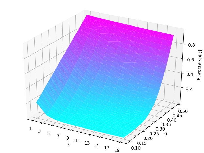
This sum cannot be simplified. But simplification is not required if we want to get an idea of how likely it is to get a worse split. We can bound the probability by observing that the values summed become very small as $i$ increases. This probability is $\Omega \left ( \alpha^{\frac{k}{2}} \right )$ and all the terms that we omitted are orders of magnitude smaller which won’t affect the probability significantly. (Note: This is dependant on $\alpha$. For instance, if $\alpha=\frac{1}{10}$, the next elements are about 10 times smaller.) I have written a script that computes this probability for several $\alpha$ and $k$. Here are the results:

As expected, it looks like picking more elements to get a better probability of a good median becomes less and less worth the increased runtime (notice how the curve along the $k$ axis, when $\alpha=0.1$, barely moves anymore when $k > 5$).

I want guarantees

What if we wanted a guarantee on the behavior of quicksort ? What if we selected the true median with a common algorithm like median-of-median that runs in $O(n)$. That would not change the time complexity of the algorithm but it would heavily impact the runtime of the algorithm nonetheless, because of the hidden constants. Given the previous results, it is deemed better to fallback to a simple median strategy that yields good results most of the time and opt for other sorting algorithms like mergesort or heapsort for systems that require guarantees.

References

• Cormen, T. H., & Cormen, T. H. (2001). Introduction to algorithms. Cambridge, Mass: MIT Press.

1. $T(n) \in O(f(n)) \iff \exists c \in \mathbb{R}_+ \land \exists n_0 \in \mathbb{N} \mid 0 \leq T(n) \leq cf(n) \ \ \forall n \geq n_0$
2. $T(n) \in \Theta(f(n)) \iff \exists c_1, c_2 \in \mathbb{R}_+ \land \exists n_0 \in \mathbb{N} \mid 0 \leq c_1f(n) \leq T(n) \leq c_2f(n) \ \ \forall n \geq n_0$
3. $T(n) \in \Omega(f(n)) \iff \exists c \in \mathbb{R}_+ \land \exists n_0 \in \mathbb{N} \mid 0 \leq cf(n) \leq T(n) \ \ \forall n \geq n_0$

Notice how the $\in$ operator has been used because $O$, $\Theta$ and $\Omega$ are sets. The $=$ sign is notation abuse. This notation tells us how the algorithm will behave according to a function. In asymptotic analysis, constants are stripped from the function because we only care about the behavior of the function, its growth. Assuming that $n$ is very large, the constants will not matter when comparing two algorithms (you can think of it as a limit).This notation proved itself to be very useful for analyzing algorithms, in theory at the very least. When we are given the task of chosing an algorithm over the other, we pick the one who’s tightest time or space complexity seems to be more favorable.

I was always wondering what does the notation tell us about the growth of the input size or magnitude $n$. In the real world, we usually have a finite set of ressources. We want our algorithms to run fast and not to exceed a certain time to terminate or to hog too much memory. To accomplish a task faster, we can pick a different algorithm with a better complexity (for the given circumstances) or upgrade the hardware on which it is running. Upgrading the hardware will usually have a straightforward effect on the algorithm. All things being equal, a processor twice the clock speed of another will perform about twice faster. But how does that affect the input size or the magnitude of the algorithm’s input ? Is it ever worth upgrading hardware ? Formally,

Given an algorithm $A$ with a ressource consumption given by $T(n)$, available ressource $R$ and a speedup of $k$, how much larger can $n$ be such that $T(n) \leq R$?

In other words, if my current system runs algorithm $A$ in $R$, if I were to upgrade for a better system that would run $k$ faster, how much larger $n$ could be and still statisfy the ressource constraint. Here, $R$ is not an entirely accurate representation of the ressource consumption of an algorithm as it is difficult to map an algorithm to an exact value, with units. Rather, we are interest into the behavior of the algorithm and the magnitude of its input when ressources are finite. A speedup of $k$ means that

where $T’$ represents the ressource consumption of the new system. The objective is to determine the relationship between $n_1$ and $n_2$. We know that

With equation 1, we can deduce that

And so

With this in hand, we can substitute $T$ for any function and get our result. Here is a table of common functions:

Notice how the slowest growing functions provide the largest growing ratio of input. For exponential functions, notice how the input can barely be any larger because of the base of the logarithm (and the logarithm itself that has a slow growth, relatively speaking). Finally, it is interesting that both logarithmic and exponential functions depend on the the value of $R$. A larger $R$ makes logarithmic functions all the more worth the it whereas, as just stated, exponential functions will be severely hindered in their acceptable input size. To double the input size of an algorithm that follows an exponential growth, one would have to get a computer $R$ times faster (up to a constant of course).

In conclusion, it appears that a better algorithm will usually beat better hardware, especially when the time complexity is undesirable. But it is not always about chosing one over the other. It is evident that a better algorithm will let you do even more with better hardware. A logarithmic algorithm will perform exponentially better with better hardware. In other words, hardware upgrade is all the more justified when it runs a good algorithm.

References

• Cormen, T. H., & Cormen, T. H. (2001). Introduction to algorithms. Cambridge, Mass: MIT Press.

Divide And Conquer

Divide and conquer is a class of algorithms that aim to solve a problem by dividing it into smaller chunks and recursively solving them. Generally, once the recursion is over, there is a final step that aims to combine the result of the recursive calls into a valid output.

A common representative of this class of algorithms is merge-sort. The input list is split in half and sorted by a recursive call (until the lists have a size of 1). Once both sides are sorted, the algorithm will merge the lists into a larger sorted list. It is rather difficult not to be charmed by the elegance of these algorithms. Nowhere in the process of sorting a list with merge-sort do we explicitly sort the two halves of the list. Instead, we start from the trivial base case of the single item lists and work our way up by merging sorted lists.

Master Theorem

Divide and conquer algorithms’ performance is usually modeled by a recurrence of the following form:

where \(T(n)\) represents the time consumption of the algorithm for an input of size (or magnitude) of \(n\), \(f(n)\) represents the work accomplished within the current call to the algorithm to either split or combine the problem. \(a\) and \(b\) are constants. If we were to model the time consumption of merge-sort, we would get the following recurrence:

which can be approximated to

The Master Theorem is an approach that aims to provide an asymptotic analysis to the runtime to reccurence relations like the ones previously described. It is defined as:

Again, in the case of merge-sort, \(T(n) \in \Theta(n \log n)\) because \(n \in \Theta(n ^ { \log_22 }) = \Theta(n)\).

A Recursive Expansion

Looking at the theorem, it is difficult to intuitively make sense of the reasons behind the conditions. Before being presented to the Master Theorem, I would solve recurrences manually by expanding the equation until I got a good intuition on the end result.

The idea behind the expansion is to compare the work that is done by the current call compared to previous calls. If we take a look at each recursive call, we observe that \(a\) and \(b\) are directly affecting the asymptotic analysis of the algorithm. A larger \(a\) and a asymptotically larger \(f\) will make each recursive calls more costly whereas a larger \(b\) will reduce the amount of recursive calls.

Most proofs that I have come across tend to assume the Master Theorem is right and use a direct approach to show that it does not lead to any contradictions. I believe that this type of approach does not lead to too much insight on the underlying logic behind the three cases of the teorem. Furthermore, the Master Theorem described here defined \(f\) as an arbitrary function. Most of the time, \(f\) will be a polynomial function of the \(k^{\text{th}}\) order, that is \(f(n) \in \Theta(n^k)\), and this is how most of the intuition will come from.

We can rewrite equation 3 as such:

This sum is a geometric serie of the form \(\sum_{i=0}^k c^i = \frac{c^{k+1} - 1}{c - 1}, \ c \neq 1\) ($n^k$ was left out) where \(c = \frac{a}{b^k}\). There are three interesting cases.

1. \(c < 1 \implies a < b^k\) :

   \[\sum_{i=0}^{ \log_b n } c^i = \frac{c \cdot n^{\log_bc} - 1}{c - 1}\]

   Because \(c < 1\), \(\log_bc < 1\). As \(n\) gets larger, the sum will converge towards a constant because \(n^{\log_bc}\) converges towards \(0\). Therefore, \(T(n) \in \Theta(n^k)\).

2. \(c = 1 \implies a = b^k\). This is a trivial case. $T(n) \in \Theta(n \log n)$.

3. \(c > 1 \implies a > b^k\) :

   \[\frac{c \cdot n^{\log_bc} - 1}{c - 1} = \frac{\frac{a}{b^k} \cdot n^{\log_b{\frac{a}{b^k}}} - 1}{\frac{a}{b^k} - 1} \in \Theta(n^{\log_ba - k})\]

And so $T(n) \in \Theta(n^{\log_ba})$. In order to prove that we have in hand the Master Theorem itself, it is required to describe the the relationship between $f(n) = n^k$ and constants $a$ and $b$. For the first case, we stated that

In order to make $f(n)$ appear, $k$ must be isolated:

And there we have it, the third case of the theorem. The two others can be derived the same way. The Master Theorem is no longer the intimidating theorem that it used to be. It all came down to a geometric serie with three interesting edge cases.

Note: This is by no means a proof to the theorem. The assumption on $f$ being a polynomial function does not cover all the cases.

References

• Cormen, T. H., & Cormen, T. H. (2001). Introduction to algorithms. Cambridge, Mass: MIT Press.